TL;DR
- MAPE is the most common forecast accuracy metric, but it breaks down when actuals are low or zero — which is exactly when operators need accuracy most.
- WAPE solves MAPE's volume-bias problem by weighting errors proportionally. It is the metric finance teams should standardize on.
- Bias measures whether you systematically over-forecast or under-forecast. A forecast can have low error (good MAPE) and high bias (systematically wrong direction) at the same time.
- The metrics finance trusts go beyond single-number accuracy: they include segment-level variance, confidence intervals, and week-over-week trend.
- Accuracy improves with process, not tools alone: weekly measurement, segment-level tracking, CRM hygiene, and structured rep judgment are the four levers that move the number.
Most sales forecasts are wrong. The question is not whether your forecast will miss — it is whether you know by how much, in which direction, and whether the error is random noise or a systematic bias you can fix. Sales forecasting without accuracy measurement is not forecasting. It is hoping with a spreadsheet.
This post covers the metrics that separate a forecast finance trusts from one they discount before the meeting starts. You will get the formulas for MAPE and WAPE, the limitations most teams discover too late, a clear method for detecting bias, and five process changes that improve accuracy within a quarter — without buying new software.
---Why Forecast Accuracy Matters
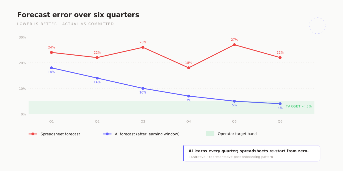
A forecast that is consistently 20% off is not a forecasting problem. It is a planning problem, a hiring problem, a cash management problem, and often a board-credibility problem rolled into one.
When a forecast overestimates revenue by 20%, the business plans spend it does not have. Marketing budgets get committed. Headcount gets approved. Inventory gets ordered. The correction, when it comes, is painful. When a forecast underestimates by 20%, the business under-invests. Opportunities get missed. Competitors capture market share that should have been defended.
The cost of forecast error is not abstract. Research from the Institute of Business Forecasting found that a 1% improvement in forecast accuracy can reduce inventory carrying costs by 1.5–3% and improve perfect order rates by a comparable margin. For a $10M ARR business, moving from ±15% forecast error to ±5% translates into more predictable cash flow, better supplier terms, and fewer emergency decisions made under pressure.
Accuracy measurement also changes behavior. Teams that track forecast error weekly improve faster than teams that review accuracy quarterly. The act of measuring creates accountability. Reps who know their commits will be compared to actuals within 7 days submit more realistic numbers. Managers who see segment-level error rates know which part of the pipeline to inspect.
The first step to improving forecast accuracy is choosing the right metric. Most teams start with MAPE. Many should stop there and switch to WAPE.
---MAPE (Mean Absolute Percentage Error)
MAPE is the most widely cited forecast accuracy metric. It is simple to calculate, easy to explain, and produces a single percentage that anyone in the business can understand. That accessibility is also its trap.
Formula
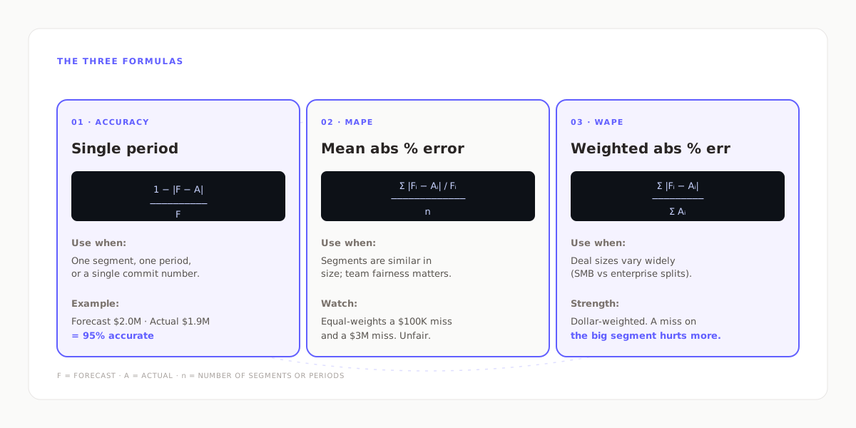
MAPE = (1/n) × Σ |Actual − Forecast| / Actual × 100
Where n is the number of periods, and the sum is taken across all periods.
How to calculate it step by step:
- For each period (week, month, quarter), subtract forecast from actual. Take the absolute value. This gives you the absolute error for that period.
- Divide the absolute error by the actual value for that same period. This gives you the percentage error for that period.
- Repeat for all periods in your dataset.
- Sum all percentage errors and divide by the number of periods.
- Multiply by 100 to express as a percentage.
A worked example:
| Week | Actual | Forecast | |Error| | % Error |
|---|---|---|---|---|
| Week 1 | $50,000 | $45,000 | $5,000 | 10.0% |
| Week 2 | $80,000 | $92,000 | $12,000 | 15.0% |
| Week 3 | $35,000 | $30,000 | $5,000 | 14.3% |
| Week 4 | $120,000 | $108,000 | $12,000 | 10.0% |
| Total / Average | $285,000 | $275,000 | $34,000 | 12.3% |
In this example, MAPE = (10.0 + 15.0 + 14.3 + 10.0) / 4 = 12.3%. The forecast is off by an average of 12.3% per week.
When MAPE works:
- Your actuals are consistently high-volume — no period is near zero.
- Your product portfolio is homogeneous — you are forecasting one product or one segment.
- You need a metric that non-technical stakeholders can understand immediately.
When MAPE fails:
- Low-volume periods: If actual is $2,000 and forecast is $2,500, the absolute error is $500 — small in dollar terms — but MAPE reports 25%. One low-volume week can distort your entire accuracy score.
- Zero actuals: MAPE is undefined when actual equals zero (division by zero). This happens more often than most teams expect — new product launches, seasonal slowdowns, or accounts going dormant.
- Mixed portfolios: If you forecast ten products and average their MAPEs, a low-revenue product with 50% error gets the same weight as a high-revenue product with 5% error. The aggregate MAPE does not reflect the economic significance of each miss.
These limitations are not edge cases. They are the normal operating conditions of most B2B sales forecasts. That is why finance teams increasingly prefer WAPE.
---WAPE (Weighted Absolute Percentage Error)
WAPE solves the problems that make MAPE unreliable in real business conditions. It is volume-weighted, handles low-volume periods gracefully, and produces the same result whether you calculate at the item level or the aggregate level. For operators running multi-product or multi-segment forecasts, WAPE is the better standard.
Formula
WAPE = Σ |Actual − Forecast| / Σ Actual × 100
Where both sums are taken across all periods or all items in the dataset.
The difference from MAPE is in the order of operations:
- MAPE calculates a percentage for each period, then averages the percentages.
- WAPE sums all absolute errors first, then divides by the sum of all actuals.
This means WAPE weights each period by its volume. A $500 error on a $50,000 week contributes 1% to WAPE. A $500 error on a $2,000 week contributes 25% to WAPE. The metric automatically reflects the economic significance of each miss.
The same worked example, calculated as WAPE:
| Week | Actual | Forecast | |Error| |
|---|---|---|---|
| Week 1 | $50,000 | $45,000 | $5,000 |
| Week 2 | $80,000 | $92,000 | $12,000 |
| Week 3 | $35,000 | $30,000 | $5,000 |
| Week 4 | $120,000 | $108,000 | $12,000 |
| Total | $285,000 | $275,000 | $34,000 |
WAPE = $34,000 / $285,000 × 100 = 11.9%
In this example, MAPE and WAPE are close because the volumes are relatively balanced. The divergence becomes dramatic when volumes vary widely or when low-volume periods are present. In a typical B2B forecast with seasonal dips and multi-product portfolios, WAPE and MAPE can differ by 5–15 percentage points.
When to use WAPE:
- You forecast a mixed portfolio of products, segments, or regions with different volume levels.
- Your business has low-volume periods where MAPE would distort the score.
- You need a metric that is mathematically consistent whether calculated at the item level or rolled up to the total.
- You report forecast accuracy to finance, who care about dollar-weighted error, not per-period percentages.
WAPE's limitation: Like MAPE, WAPE is undefined when the sum of actuals is zero. This is rare in practice — it would require every period in your dataset to have zero actuals — but worth noting for new product launches before the first sale closes.
---Bias: Detecting Systematic Over-Forecasting and Under-Forecasting
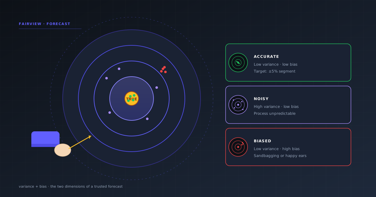
A forecast can have low error and high bias at the same time. This is the most dangerous combination — the forecast looks accurate on average, but it is consistently wrong in the same direction. Finance learns to discount it. Reps learn to pad or sandbag. The forecast becomes theater.
Bias measures the direction of error, not just the magnitude. A positive bias means you over-forecast (forecast > actual). A negative bias means you under-forecast (forecast < actual). Random error averages to zero over time. Bias does not.
Formula
Bias = Σ (Forecast − Actual) / Σ Actual × 100
Positive = over-forecasting. Negative = under-forecasting. Zero = unbiased.
How to interpret bias:
| Bias Range | Interpretation | Typical Cause |
|---|---|---|
| +10% or higher | Severe over-forecasting | "Happy ears" — reps overestimate close probability |
| +5% to +10% | Moderate over-forecasting | Optimistic stage weights or inflated pipeline |
| −5% to +5% | Acceptable range | Normal random variation |
| −10% to −5% | Moderate under-forecasting | Sandbagging or conservative commit culture |
| −10% or lower | Severe under-forecasting | Fear of missing quota; deals hidden until certain |
Track bias on two time horizons:
- 4-week rolling bias: Catches recent shifts in rep behavior or market conditions. A sudden move from +2% to +8% bias signals that something changed in the past month.
- 12-week rolling bias: Reveals structural patterns. If 12-week bias stays above +5% for two consecutive quarters, your forecasting methodology — stage weights, close-date assumptions, or rep judgment — needs revision.
The bias-accuracy combination matrix:
| Low Bias (±5%) | High Bias (>±10%) | |
|---|---|---|
| Low Error (<10%) | Ideal: accurate and unbiased | Dangerous: looks accurate, consistently wrong direction |
| High Error (>20%) | Noisy but centered: process issue, not behavioral | Broken: wrong direction and large magnitude |
The bottom-right quadrant — high error and high bias — is where most broken forecasts live. The top-right quadrant is more insidious: the forecast appears accurate because errors cancel out, but the direction is systematically wrong. Finance spots this quickly. Operators should spot it first.
---The Metrics Finance Actually Trusts
MAPE, WAPE, and bias are the foundation. Finance teams with mature forecasting processes layer three additional metrics on top. These metrics answer questions that single-number accuracy cannot.
1. Segment-level variance
Aggregate accuracy hides segment-level problems. A forecast that is ±3% overall can be ±25% in enterprise deals and ±40% in self-serve. Without segment-level tracking, you do not know where to focus improvement efforts.
Calculate WAPE separately for each segment you forecast: by product line, by deal-size band, by region, by rep tenure, by lead source. The segment with the highest error rate is where your next process improvement should land. In our experience, 60–70% of total forecast error comes from one or two segments. Fixing those segments moves the aggregate number faster than marginal improvements everywhere.
2. Confidence intervals (optimistic vs. conservative range)
A single-point forecast — "we will close $400K" — is almost always wrong. A range forecast — "we will close between $340K and $460K, with $400K as the most likely outcome" — is more honest and more useful.
Finance trusts forecasts that include a confidence range. The width of the range signals forecast maturity: narrow ranges indicate high confidence (and high risk if missed), while wide ranges indicate acknowledged uncertainty. Track how often actuals fall inside the stated range. A forecast that lands inside its own confidence interval 70–80% of the time is well-calibrated. Below 50% means the range is too narrow.
3. Week-over-week forecast drift
Track how much the forecast for the same period changes as the period approaches. If your Q3 forecast moves from $1.2M to $900K to $1.1M between July 1 and September 15, the early forecast is not providing value. It is creating noise.
Measure drift as the coefficient of variation (standard deviation of weekly forecast values divided by the mean) for each period. A drift coefficient above 0.15 indicates an unstable forecasting process. The goal is not zero drift — new information should update the forecast — but drift that shrinks as the period approaches and stabilizes in the final 2–3 weeks.
4. The tracking signal
The tracking signal is a running indicator of whether your forecast is drifting into bias territory. It is calculated as the cumulative sum of forecast errors divided by the mean absolute deviation.
Formula
Tracking Signal = Σ (Forecast − Actual) / MAD
Where MAD = mean absolute deviation = Σ |Forecast − Actual| / n
A tracking signal between −4 and +4 indicates normal variation. Values outside ±6 suggest the forecast model is no longer appropriate for the current environment — either the market has shifted or the methodology has broken down.
---5 Ways to Improve Forecast Accuracy (Starting This Week)
Tools help. Process helps more. The teams that move from ±15% to ±5% accuracy do not typically buy new software. They change how they measure, review, and act on the forecast.
1. Measure accuracy weekly — not monthly or quarterly
Most teams review forecast accuracy at the end of the quarter. By then, the patterns that caused the miss are buried under three months of new data. Weekly measurement creates a tight feedback loop. Reps see their error within 7 days. Managers spot drift before it compounds. The habit of measuring is more valuable than the specific metric you choose.
Start with a simple spreadsheet: four columns (week, actual, forecast, error percentage). Calculate WAPE on a 4-week rolling basis. Share the number in the weekly revenue review. Within 4–6 weeks, the act of publishing the number will change how reps think about their commits.
2. Track accuracy by segment, not just in aggregate
Aggregate accuracy is a summary, not a diagnosis. Break your forecast into the segments that matter: by product line, by deal size, by sales stage, by rep tenure, by lead source. Calculate WAPE and bias for each segment separately.
The pattern is almost always the same: 2–3 segments drive 70% of the total error. One segment might have a +18% bias (systematic over-forecasting). Another might have 35% WAPE (high variance). Fix those two segments and the aggregate number improves disproportionately.
3. Enforce CRM hygiene as a forecasting prerequisite
A forecast is only as good as the data it is built from. Deals not logged in the CRM are invisible to any forecasting method. Close dates that are never updated produce phantom pipeline. Stage definitions that vary by rep make stage-based weighting meaningless.
Before investing in a new forecasting method, audit your CRM data quality:
- What percentage of deals have a close date within the forecast period?
- What percentage of deals have been updated in the past 14 days?
- How consistent are stage definitions across reps?
- What is the match rate between CRM close dates and actual invoice dates?
If data quality is below 80% on any of these dimensions, fix the data before you fix the forecast model. A sophisticated model running on dirty data produces a sophisticated wrong answer.
4. Implement structured rep judgment, not open-ended commits
Rep judgment is one of the most accurate inputs to a forecast — when it is structured. Open-ended questions ("how much will you close?") produce optimistic answers. Structured judgment produces calibrated answers.
Ask reps to provide three numbers, not one:
- Best case: Everything goes right. Deals close early. No pushbacks.
- Most likely: The outcome you would bet on if you had to.
- Commit: The number you are confident you will hit, even if one or two deals slip.
Track each rep's historical accuracy on each of these three numbers. Some reps are consistently optimistic on "most likely." Others are conservative on "commit." Knowing each rep's bias pattern lets you apply a correction factor — not to punish, but to improve the forecast.
5. Review forecast error in the weekly operating rhythm
The forecast review should include two questions every week:
- What changed in the forecast this week, and why?
- How accurate was last week's forecast for the period that just closed?
The first question catches drift. The second question builds accountability. Over time, the team learns which signals predict accuracy and which signals are noise. The forecast improves not because the model changed, but because the people using it learned.
---How Fairview Tracks Forecast Accuracy
Fairview's Forecast Confidence Engine is built around the principle that a forecast without an accuracy score is not a forecast — it is a target dressed in probability language. The engine connects to your CRM (HubSpot, Salesforce, or Pipedrive) through the Data Connection Layer, reads deal stage, close date, and historical close rates, and produces a confidence-weighted revenue forecast every week.
What the Forecast Confidence Engine does:
- Generates a weekly revenue forecast based on pipeline stage, historical close rates, and deal velocity from your connected CRM data.
- Assigns a confidence score (High / Medium / Low) based on pipeline composition — the mix of deal stages, the concentration of value in a few large deals, and the recency of rep activity.
- Shows an optimistic-to-conservative range, not a single number. Finance sees the full distribution, not a point estimate.
- Compares actual-to-forecast week over week, calculating WAPE and bias automatically and surfacing the trend in the Weekly Operating Report.
How accuracy tracking shows up in practice:
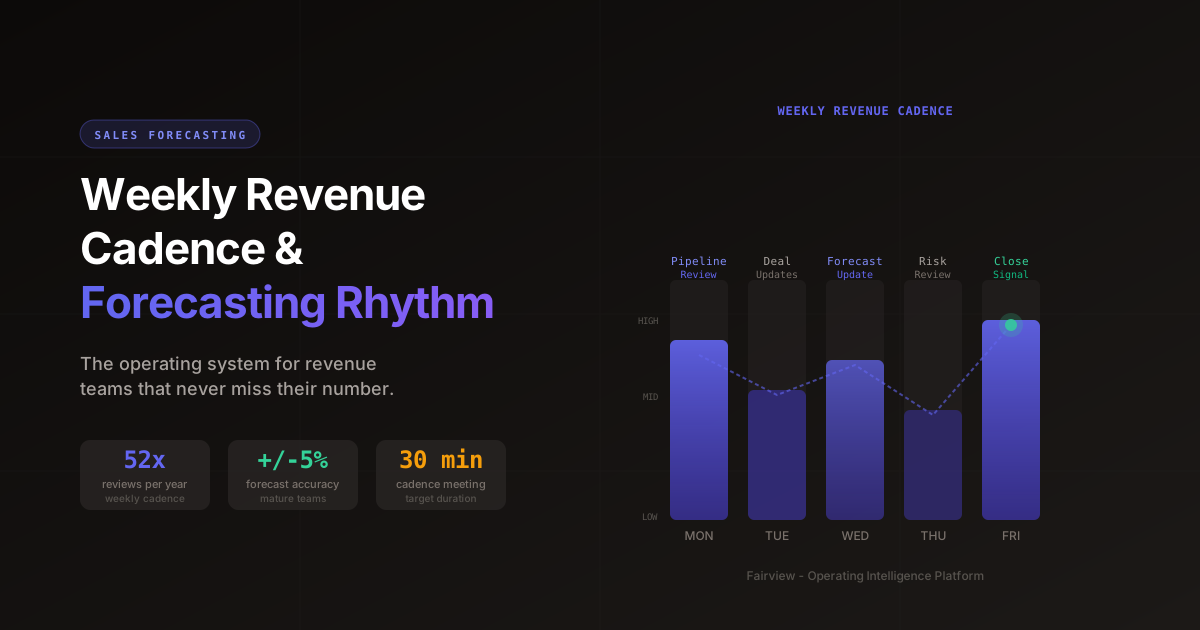
Every Monday morning, the Weekly Operating Report arrives in the operator's inbox. It includes revenue vs. forecast for the prior week, the rolling 4-week WAPE, the 12-week bias trend, and a flag if either metric has moved outside the acceptable range. The operator arrives at the weekly review already briefed on whether the forecast is improving, stable, or degrading — and which segment is driving the change.
The Pipeline Health Monitor complements the forecast by surfacing deals that are stalling — no activity in a configurable number of days, close dates slipping — before they become forecast surprises. A deal that goes quiet in Stage 4 is a signal that the forecast number attached to it may not materialize. Catching that signal early prevents the end-of-quarter miss that no amount of accuracy measurement can fix retroactively.
Fairview does not replace the judgment of experienced operators or finance teams. It automates the measurement, surfaces the patterns, and recommends the next action — so the operator's time goes into decisions, not into assembling and reconciling forecast data.
---What is a good MAPE score?
A MAPE below 10% is considered highly accurate, 10–20% is good, 20–50% is reasonable, and above 50% indicates an unreliable forecast. These benchmarks vary by industry — consumer goods with stable demand patterns often achieve sub-10% MAPE, while B2B SaaS with long sales cycles typically operates in the 15–30% range. The more important question is whether your MAPE is improving over time.
Why does MAPE fail with low-volume forecasts?
MAPE divides absolute error by actual value, so when actuals are small — say $2,000 actual vs. $2,500 forecast — the percentage error is 25% even though the dollar miss is only $500. A single low-volume period can distort your entire accuracy score. WAPE solves this by dividing total absolute error by total actuals across all periods, so low-volume periods receive proportionally less weight.
How do you detect bias in a sales forecast?
Calculate forecast bias as the sum of (forecast minus actual) divided by the sum of actuals, expressed as a percentage. A positive bias means you consistently over-forecast. A negative bias means you consistently under-forecast. Track bias over rolling 4-week and 12-week windows. A bias that persists beyond ±5% for two consecutive quarters indicates a structural problem in your forecasting process, not random error.
How long does it take to improve forecast accuracy?
Most teams see measurable improvement in 6–12 weeks if they implement structured changes: weekly forecast reviews, segment-level tracking, and CRM hygiene discipline. Moving from ±15% to ±5% accuracy typically takes one to two quarters of consistent process improvement. The key is measuring accuracy weekly — without a measurement cadence, you cannot tell which changes are working.
What is the difference between MAPE and WAPE?
MAPE calculates the percentage error for each individual period and then averages those percentages. WAPE sums all absolute errors first, then divides by the sum of all actuals. This means WAPE weights each period by its volume, preventing low-volume periods from distorting the overall score. WAPE is also mathematically simpler and produces the same result regardless of whether you aggregate before or after calculating error.
Should I track forecast accuracy by segment or in aggregate?
Track both. Aggregate accuracy tells you whether your overall forecast is trustworthy. Segment-level accuracy tells you where the error lives — which product lines, regions, or deal-size bands are driving the miss. A forecast that is ±3% in aggregate can hide a segment that is ±40% off. Segment-level tracking is the fastest way to find the specific part of your process that needs fixing.
Key takeaways
- MAPE is the most common forecast accuracy metric, but it distorts when actuals are low or zero. WAPE is the better standard for most B2B forecasts because it weights errors by volume.
- Bias measures direction, not just magnitude. A forecast with low error and high bias looks accurate on average but is systematically wrong. Track bias on 4-week and 12-week rolling windows.
- Finance trusts forecasts that include segment-level variance, confidence intervals, and week-over-week drift tracking — not just a single accuracy percentage.
- The five fastest ways to improve accuracy: measure weekly, track by segment, enforce CRM hygiene, structure rep judgment with three-number commits, and review error in the weekly operating rhythm.
- A forecast without accuracy measurement is not forecasting. The act of measuring — and publishing the number — changes behavior faster than any model improvement.
If your team is ready to move from forecasting by intuition to forecasting with measured accuracy, Fairview connects your CRM data to a confidence-weighted forecast with automatic WAPE and bias tracking — delivered in your Weekly Operating Report every Monday morning. Book a demo to see how the Forecast Confidence Engine works with your pipeline data.